PostgreSQL Stories: Taking Random Samples from Big Tables

We often see customers pull data from their Render-managed PostgreSQL database for data science and AI. Sometimes, they’re doing one-off analysis, and sometimes they’re training generative AI models. For these use cases, you often need or want to take a random sample of data. However, sampling can be slow if a database table has billions of rows, or if two large tables must be joined before you sample. Recently, we helped one of our customers resolve these exact problems. In this post, we share our findings with you. You’ll learn how to randomly sample large datasets in PostgreSQL while keeping your queries performant. Instead of telling you “the answer,” we’ll walk through possible solutions and their tradeoffs, and help you build a deeper understanding of databases. We’ll cover:

• What the top Stack Overflow answers get wrong: The most popular answer is not always the most efficient.
• Benefits and tradeoffs of nondeterministic algorithms: We introduce Bernoulli sampling and TABLESAMPLE, which are fast but come with potential downsides.
• How to use a simulation to build intuition: We walk through a simulation of 10k trials of TABLESAMPLE, which provides you with a concrete example of its tradeoffs.

Why take a random sample?

Before we dive into how to randomly sample from PostgreSQL, let’s consider why we might do it. Using a portion of data can make a large dataset more practical to use. And by taking a random sample, your sample will be statistically representative. Therefore, using a random sample can:

• Enable and accelerate model training: When you’re building a proof-of-concept for a machine learning model, you might not have enough compute resources to train on the entire dataset. Training on a smaller, random sample can speed up your development. Sampling is also a necessary step in training via stochastic gradient descent (regardless of the model and total training data size).
• Avoid overfitting in a model: Training on a random sample can help prevent overfitting by exposing the model to a variety of data points.
• Alleviate resource constraints: Large datasets can exceed the memory capacity of most machines—and we mean personal laptops as well as database servers. By sampling data, you reduce load on your system, so you can perform computations that would otherwise be infeasible.
• Enable exploratory data analysis: Working with a random sample lets you more quickly uncover patterns in data and test a hypothesis. You save time because you aren’t processing the entire dataset.

Considering these benefits, can you think of any tables in your database you’d want to sample? Note that when sampling a large dataset, you likely want to use a read replica of your PostgreSQL database.

Intuitive but inefficient: ORDER BY random()

Let’s start out with the most intuitive, but naive solution. Let’s say you’ve picked a table, my_events, and you want to sample 10k rows. You might tell the database to randomly "shuffle" the data you'd like to select from, then take 10k elements from the head of the shuffled list. This approach ranks at the top of many related Stack Overflow posts: Unfortunately, this approach is very inefficient. To understand why, let’s look at the query plan for an example run.

Our example dataset

For the analysis and query plans in this post, we've constructed the sample_values table by creating a one-column table and inserting a billion rows: Note that 10k rows represents just 0.001% of the total data.

Analyzing ORDER BY random()

Using the sample_values table, let’s analyze the naive ORDER BY random() approach: As we expected, the resulting query plan is abysmal:

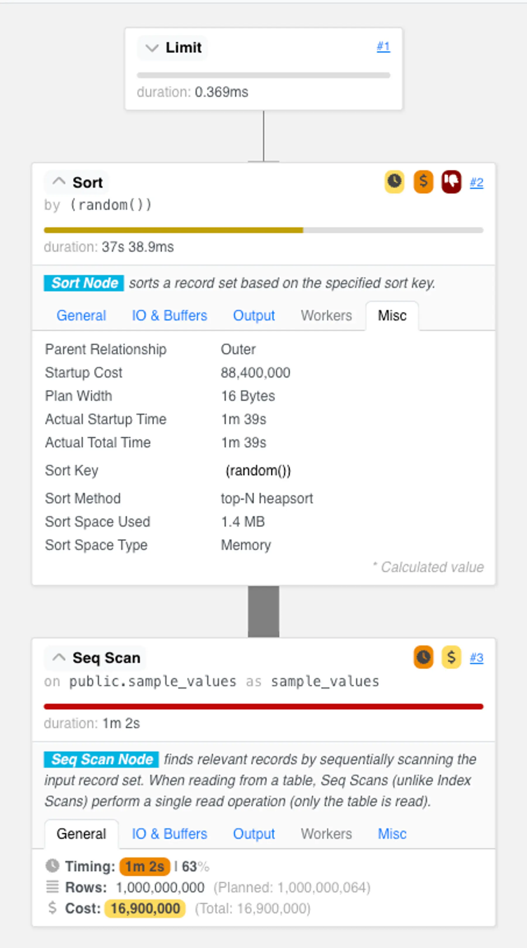
This plan has two heavyweight steps:

• It first examines every row in the table. To select just 0.001% of our data, this plan scans all billion rows. In our “best case scenario” demo environment—with no table bloat, no updated or deleted tuples we need to skip based on transaction visibility, and no concurrent clients using shared buffer resources—this scan already takes over a minute. That's eons for the computers of today!
• It then performs over 13 billion comparisons for a top-N heapsort. The top-N heapsort maintains a fixed-sized heap data structure that holds up to 10k rows that have had the lowest random() values encountered. When a new row is pulled from the table scan, it is inserted into the heap, which takes around log_2(10,000) comparisons against existing heap elements. When the heap is full, this insertion will cause the highest value to fall out of the set of candidates. After seeing all billion rows, the heap contains the sampled rows ready to be streamed to the user.

Bernoulli sampling removes costly comparisons

To improve this query plan, let’s eliminate the top-N heapsort, so we look at each row only once. In the naive plan, we first paired every row with a random value, then used those random values to compare and select rows. In the improved plan, let’s look at each row once, independently, and determine using a “dice roll” if a row should be selected. Here’s what it looks like as a database query: This technique is called Bernoulli sampling. Its efficiency comes with a trade-off: the number of rows in the output is non-deterministic. In other words, you can expect to get about 10k rows, but not exactly 10k rows, each time you sample.

Analyzing Bernoulli sampling

If we look at the query plan for the Bernoulli sampling approach, we see the runtime has decreased by 50%. Notably, this query runs in a single step, and no longer requires maintaining a secondary data structure or comparing elements. Unfortunately, it still takes over 45 seconds. The table scan is costly because it fetches a massive number of data pages into memory. In PostgreSQL, these fetches are necessary even when using a relatively efficient index scan, because visibility information is stored in the heap. (For the same reason, simply counting rows in a large table can be slow.) So, how can we further chop down the runtime?

Heap blocks to the rescue

To get even better performance, we need a way to avoid looking at every row. Fortunately, table rows in PostgreSQL are organized into groups called heap blocks. Each block is about 8kB, including some bookkeeping information such as the visibility information mentioned above. Using heap blocks, we can randomly select blocks of rows instead of individual rows. Instead of generating a random value for each row, as we did in the naive ORDER BY random() approach, we can generate a random value for each block. Then we can select or discard all rows within a block. The key win is that we only scan rows within blocks we select. When our target sample size is much smaller than the total size of the table, this new approach ends up not scanning the vast majority of the rows.

TABLESAMPLE cuts a minute to milliseconds

To put the heap blocks approach into practice, we can use a method called TABLESAMPLE. TABLESAMPLE helps us get around the fact that PostgreSQL doesn't directly expose heap blocks directly to the user. Thankfully, the SQL:2003 standard introduced TABLESAMPLE to sample blocks as we described, and PostgreSQL implements it. You can use TABLESAMPLE together with the SYSTEM table sampling method, which chooses each block with equal probability. Here’s how we might query our sample_values now: Here’s a conceptual illustration of what happens under the hood:

Aside: Using BERNOULLI instead of SYSTEM

As an alternative to SYSTEM, there's another built-in table sample method called BERNOULLI, which basically performs the same approach that we took in our WHERE random() < $percentage query earlier.

As you might expect, using this sample method is slower. It achieves a similar runtime as our WHERE random() < $percentage query.

Analyzing TABLESAMPLE

The query plan for the TABLESAMPLE query is radically different. The entire query outputs ~10k rows in about 50ms. Notably, this query, like the Bernoulli sampled query, is non-deterministic. You should expect the number of rows returned to vary. This technique comes with an additional trade-off: individual rows are no longer independently selected. All rows within a block are selected together, so if you happen to select the same block multiple times across several samplings, it means the same set of rows is selected together each time. That being said, how much of a problem is this in practice? To find out, we ran a simulation.

Exploring bias in TABLESAMPLE through a simulation

In our simulation, we ran TABLESAMPLE many times on the same dataset. This helped us better understand two things:

• Bias: We looked at how often the same heap blocks were selected. This helped us understand how much bias is introduced by selecting blocks instead of individual rows.
• Non-determinism: We looked at how many rows were returned by each TABLESAMPLE query, and at the total runtime. This helped us build intuition around what to expect from the non-deterministic output.

Specifically, we used TABLESAMPLE to select ~100k rows out of 1 billion rows, and we ran this selection 10k times.

Results when selecting ~100k rows

First, let’s talk about bias. In the combined output of our 10k trials, only ~12% of rows in the output appeared more than once. In general, we’d expect that selecting from even larger tables (with a greater number of heap blocks) will bring this percentage down. Note that the size of the rows in the table also influences the number of rows in each block. The bigger each row is, the fewer rows will fit in each block, and thus a smaller number of rows will be selected together. In other words, we’d also expect the percentage of rows that are selected more than once to be lower in tables with bigger rows. 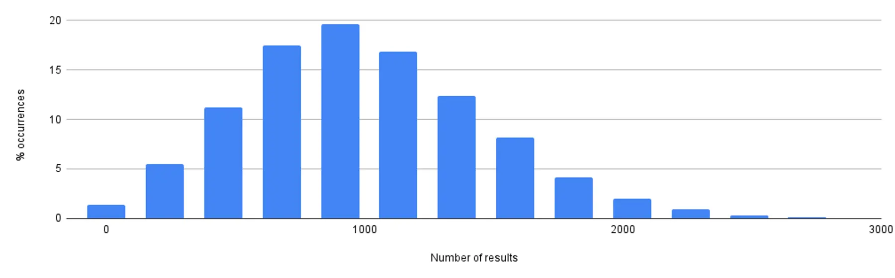Now, let’s look at nondeterminism. Our graphs showed that:

• Total runtime followed a normal distribution.
• The number of results followed a normal distribution around the target sample size (100k elements).

Selection of ~100k rows

More data on non-determinism

To further build intuition around the shape of the non-deterministic output, we also ran the trial with samples of ~1k and ~10k rows. Selection of ~1k rows

Selection of ~10k rows

Taken together, these graphs show:

• Total runtime (which also includes consuming all rows from a remote database), even for a sample size of ~100k, stays efficient. Most queries finish in under 150ms.
• The number of results all follow a normal distribution around the target sample size.

Sampling from JOIN results

Now you know a few ways to randomly sample a table. In the real world, though, we often don’t want to sample a simple table. Sometimes we want to sample the result of a join. Applying our first naive approach to a join, we’d get a query like this: How do we use the faster TABLESAMPLE technique in this situation? Let’s think about this conceptually. We could first sample from one side of the relation, then simply apply the join as a second step. We’d get a query like this: Note, this query uses a WITH clause for readability. Broadly speaking, this query works. But there are important details to note depending on the join relationship between the tables.

How JOIN relationships affect sampling

There are three general types of join relationships: one-to-one, many-to-one, and many-to-many. Here’s what to note about each type when you’re applying the query we just introduced. One-to-one: The above query will be sufficient, and you can run the TABLESAMPLE SYSTEM step on either of the two tables. It makes no difference because every row in one table matches exactly one row in the other table. Many-to-one: In this case, it does matter which table you sample from. You may want to sample from the larger (the “many” side) of the relation. Then, each sampled row joins against a single other row in the join step.

Many-to-many: Many-to-many relations may require additional sampling steps, but it really depends on your data. Often, sampling from one particular side of the relation cuts down the number of candidate rows sufficiently. You may be able to simply join against the other table, then run an ORDER BY random() to cut the joined rows down to your desired sample size.

Aside: Avoid this pitfall

We want to flag an easy way to go wrong when sampling a join. You might be tempted to run the TABLESAMPLE on both tables, like this: This query is likely not what you want. In fact, it will return zero rows most of the time. This is because you're independently sampling rows from x and y, and the rows you’ve sampled from x likely don’t join against the rows you’ve sampled in y!

Next steps

You’re now ready to sample some data from your PostgreSQL database! If you enjoyed this post, check out our PostgreSQL performance troubleshooting guide for more tips. Bookmark it for the next time you're debugging slowness or optimizing a query. You may also like the other posts in this series:

• A simple query with a big problem
• From slow query to fast—via stats